Living draft. This chapter presents the classification that gates every measure in Parts II to IV. Later chapters refer to the types by number in their Caveats sections. All example signals are synthetic; the code is shown under each figure and is MIT licensed. Found an error? Use the Report an issue link in the sidebar.
3.1 Why signal typing comes first
F0 is the rate at which a cyclic waveform repeats. An aperiodic signal has no repeating waveform and therefore has no F0 (Baken and Orlikoff 2000, 152). Jitter, shimmer and harmonics-to-noise ratio all start from an identified F0 or period, so they inherit this limit. The acoustic signals of many voice disorders do not have a periodicity that allows automatic measurement of F0 or of cycle amplitudes (Ludlow et al. 2018, 378).
Analysis software does not protect the user from this. A computer-based system may calculate a putative F0 for any signal, even an aperiodic one, and the number it displays need not have any meaning (Baken and Orlikoff 2000, 152). Checking the signal is the user’s responsibility. It is often skipped: Ludlow, Kent and Gray report a finding by Behrman (2005) that 60 % of clinicians using acoustic analysis did not examine the voice signal first to see whether periodic analysis was possible (Ludlow et al. 2018, 378).
Signal typing is that check. It sorts voice signals by how periodic they are over the interval to be analysed, so that each measure is applied only where it is valid.
3.2 Origin
The classification comes from the Workshop on Acoustic Voice Analysis, whose summary statement was written by Titze. The participants called a voice Type 1 when the periods and amplitudes of vibration are easily identified in the acoustic signal, and used Types 2 and 3 for the irregular signals typical of voice disorders (Ludlow et al. 2018, 378). Baken and Orlikoff adopted Titze’s three categories for clinical use and added subtypes within each (Baken and Orlikoff 2000, 152). Sprecher and colleagues (2010) later tested whether the types could be identified from narrowband spectrograms. They found four categories, splitting noise-dominated signals off from Type 3 as a new Type 4 (Ludlow et al. 2018, 378).
3.3 The types
The definitions and subtypes for Types 1 to 3 are those of Baken and Orlikoff. Their subtypes are shown in italics.
3.3.1 Type 1: nearly periodic
Nearly periodic (or, in the ideal case, periodic) waveforms that do not undergo qualitative changes during the interval analysed. Any modulating or subharmonic frequencies present have at least one order of magnitude less energy than the fundamental (Baken and Orlikoff 2000, 152).
Subtype A: minor random variation of F0 or waveshape.
Subtype B: minor monotonic modulation, with F0 or amplitude steadily increasing or decreasing.
Subtype C: minor cyclic variation (modulation) of F0 or amplitude.
Signals with sudden qualitative changes (bifurcations) in the interval analysed, or with modulating or subharmonic frequencies whose energy is comparable to that of the fundamental. Type 2 signals are clearly ordered and organised, but no single F0 value validly characterises the whole segment (Baken and Orlikoff 2000, 153).
A common Type 2 pattern is period doubling. Successive cycles alternate between two shapes, which puts a component at half the fundamental (F0/2) into the spectrum. The waveform then has two defensible periods: one per oscillation or one per pair (Baken and Orlikoff 2000, 151).
3.3.3 Type 3: no apparent periodicity
Signals without apparent periodicity, and hence not validly susceptible to F0 measurement. A Type 3 signal may nonetheless be chaotic, with a covert organising principle that the techniques of dynamical systems theory might reveal (Baken and Orlikoff 2000, 153).
Type 4 was added by Sprecher and colleagues for signals dominated by noise, separated from Type 3 (Ludlow et al. 2018, 378). Their example Type 4 waveform is aperiodic and is described as stochastic noise (Ludlow et al. 2018, 6).
3.4 What the types look like
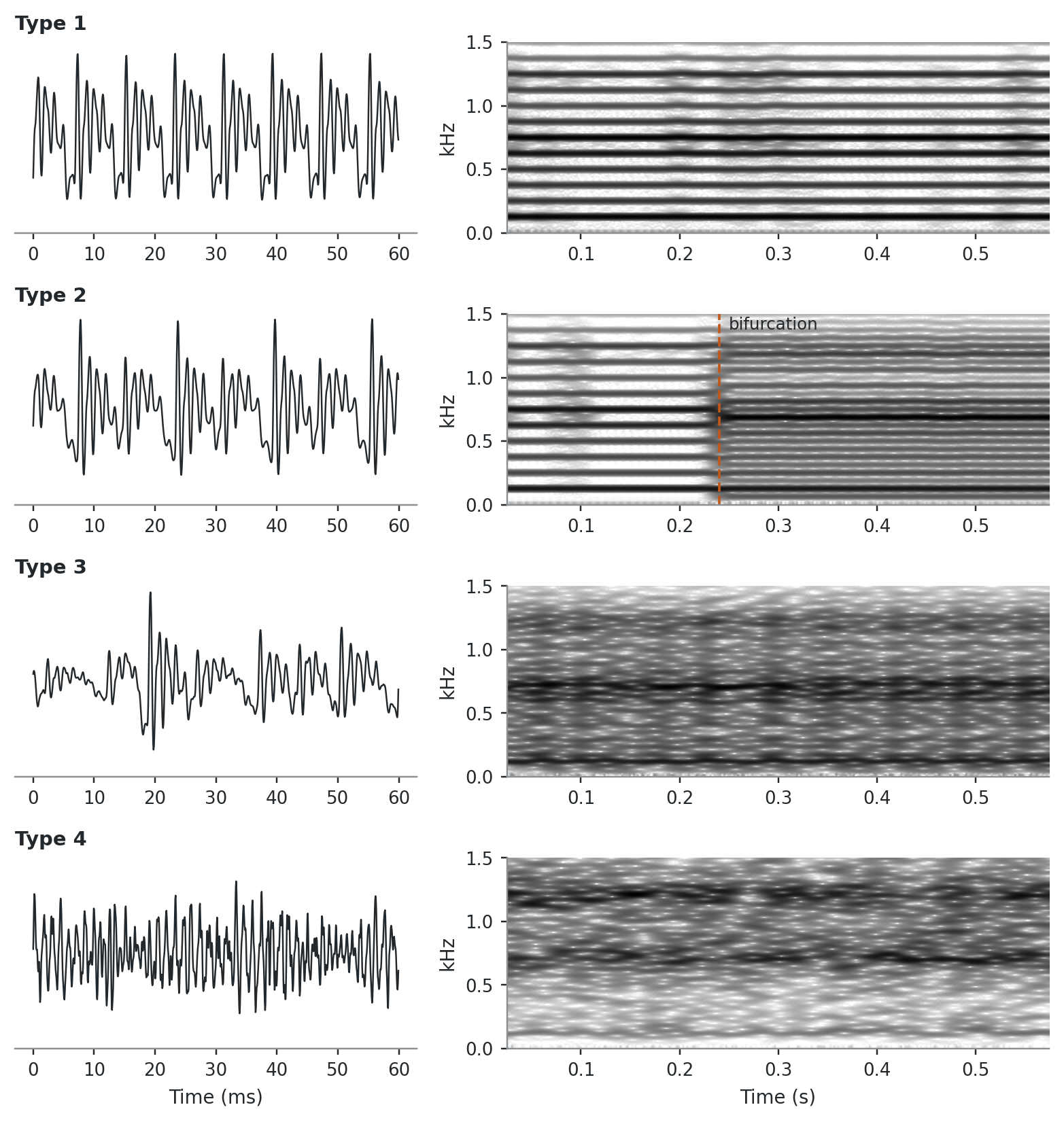
Figure 3.1 shows one synthetic example of each type. Each is a pulse train passed through the same vowel filter; only the cycle-to-cycle pattern differs. The spectrograms use a long window, so harmonics show as horizontal lines when they exist.
Figure 3.1: Synthetic examples of the four signal types. Left: 60 ms of waveform. Right: narrowband spectrogram (50-ms Hamming window, 0–1.5 kHz) of the whole 0.6-s segment. Type 1: small random period and amplitude variation; harmonics are clean lines. Type 2: a bifurcation at 0.19 s (shaded) from period-1 to period-2 behaviour; new lines appear midway between the harmonics, at odd multiples of F0/2. Type 3: cycle lengths and amplitudes driven by a deterministic chaotic map; no stable harmonic lines. Type 4: weak irregular pulses buried in noise; energy is spread across frequency.
3.5 Applying the classification
The type belongs to an analysis interval, not to a speaker or a diagnosis. Both Type 1 and Type 2 are defined by what happens during the interval to be analysed (Baken and Orlikoff 2000, 152–53), so the same phonation can contain a Type 1 stretch and a Type 2 stretch. The practical question is always whether the segment you intend to measure is Type 1.
Ludlow, Kent and Gray describe the procedure. Select a segment of a prolonged vowel that is quasiperiodic, so that the periods of vibration can be detected accurately. Examine it with a narrowband spectrogram to see whether F0 and its harmonics are visible. If they cannot be identified, the signal is probably Type 3 or Type 4 and is not suitable for perturbation analysis (Ludlow et al. 2018, 378).
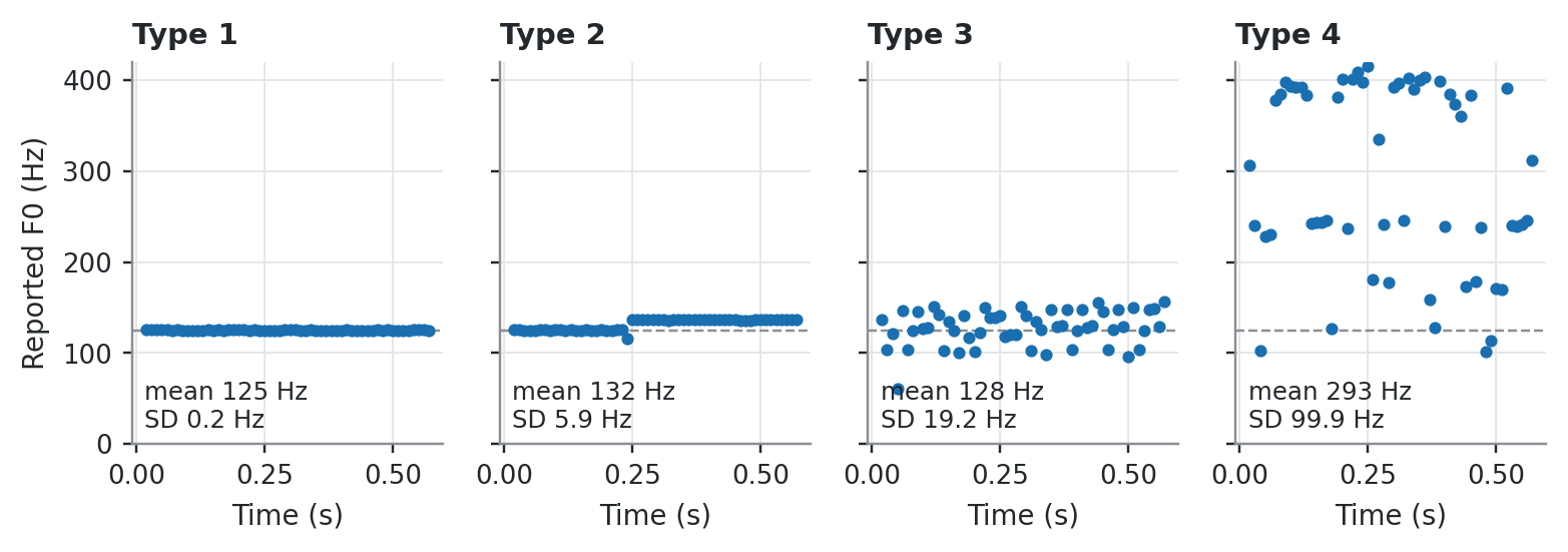
Figure 3.2 shows why the inspection cannot be delegated to the software. A simple autocorrelation F0 tracker without a voicing decision returns a value for every frame of every example. Only the Type 1 values describe the signal.
Figure 3.2: F0 returned every 10 ms by a naive autocorrelation tracker (40-ms frames, search range 60–400 Hz, no voicing decision) for the four synthetic signals of Figure 3.1. The dashed line is the 125-Hz rate of the pulse generator. Every frame gets a number. Type 1: the numbers describe the signal. Type 2: after the bifurcation the tracker settles on about 137 Hz, the rate of the shorter cycle of each pair; it describes neither the alternating pattern nor the 62.5-Hz pair rate. Types 3 and 4: the numbers are produced by the algorithm, not by any period in the signal.
flowchart TD
    A["Select a quasiperiodic segment<br/>of the sustained vowel"] --> B["Inspect the waveform and a<br/>narrowband spectrogram"]
    B --> C{"F0 and harmonics<br/>visible?"}
    C -- "No" --> G["Type 3 or 4:<br/>no F0-based measures"]
    C -- "Yes" --> D{"Qualitative change, subharmonics,<br/>or strong modulation<br/>in the interval?"}
    D -- "No" --> E["Type 1:<br/>F0, perturbation and<br/>noise measures apply"]
    D -- "Yes" --> F{"Can a shorter Type 1<br/>segment be isolated?"}
    F -- "Yes" --> A
    F -- "No" --> H["Type 2:<br/>report perturbation as<br/>not applicable"]
    G --> I["Use measures that do not<br/>need F0, such as CPPS;<br/>describe the signal"]
    H --> I
flowchart TD
    A["Select a quasiperiodic segment<br/>of the sustained vowel"] --> B["Inspect the waveform and a<br/>narrowband spectrogram"]
    B --> C{"F0 and harmonics<br/>visible?"}
    C -- "No" --> G["Type 3 or 4:<br/>no F0-based measures"]
    C -- "Yes" --> D{"Qualitative change, subharmonics,<br/>or strong modulation<br/>in the interval?"}
    D -- "No" --> E["Type 1:<br/>F0, perturbation and<br/>noise measures apply"]
    D -- "Yes" --> F{"Can a shorter Type 1<br/>segment be isolated?"}
    F -- "Yes" --> A
    F -- "No" --> H["Type 2:<br/>report perturbation as<br/>not applicable"]
    G --> I["Use measures that do not<br/>need F0, such as CPPS;<br/>describe the signal"]
    H --> I
Figure 3.3: Signal-typing workflow before measurement. Branch labels follow the definitions of Baken and Orlikoff (2000, pp. 152–153) and the inspection procedure described by Ludlow, Kent and Gray (2018, p. 378).
3.6 Which measures apply to which types
Table 3.1: What each signal type supports.
Type
F0
Perturbation (jitter, shimmer)
1
A single F0 characterises the interval. Evaluation of F0 presupposes Type 1, subtype A, within reasonable limits (Baken and Orlikoff 2000, 153).
Other measure families relate to the types as follows.
Harmonics-to-noise ratio. HNR needs a filter that separates F0 and its harmonics from the rest of the signal. Like jitter and shimmer, it can only be applied to a steady phonation such as a prolonged vowel (Ludlow et al. 2018, 378). It therefore shares their dependence on a Type 1 segment.
Cepstral peak prominence. CPP does not require direct computation of F0, and it can be extracted from connected speech as well as sustained vowels (Murton et al. 2020, 1596). Because no pitch detection or tracking is used, the cepstral measures are robust in dysphonic voices, particularly breathy ones (Barsties v. Latoszek et al. 2018, 316). The 2018 ASHA guidance recommended CPP as a general measure of dysphonia in place of jitter, shimmer and HNR (Murton et al. 2020, 1596). See the CPPS chapter.
Dynamical-systems methods. For Type 3 signals, any covert organisation might be discoverable with the techniques of dynamical systems theory (Baken and Orlikoff 2000, 153).
3.7 Caveats
Typing is a judgement. The types are defined by inspection, and the boundary between Type 1 and Type 2 is stated as an energy ratio (an order of magnitude below the fundamental versus comparable to it) (Baken and Orlikoff 2000, 152–53). None of the ingested sources reports inter-rater agreement for signal typing.
Perturbation can move the wrong way with treatment. When a voice is very irregular before treatment, few periods can be tracked, and jitter and shimmer may come out low. As the voice improves, more periods are identified and the measured values may rise (Ludlow et al. 2018, 378). Type the signal at every session before comparing perturbation values over time.
Occasional discontinuities. Occasional discontinuities may be less damaging to perturbation measurement than was once believed, at least for some software (Baken and Orlikoff 2000, 153). The requirement for a Type 1 segment still stands.
Subtypes are an extension. The A/B/C subtypes are Baken and Orlikoff’s addition to Titze’s three categories (Baken and Orlikoff 2000, 152). Cite a subtype only where the analysis depends on it.
The original sources are not yet in the library. The workshop summary statement and the Sprecher et al. (2010) paper are cited here through Baken and Orlikoff (2000) and Ludlow et al. (2018).
3.8 Points of disagreement
Date of the classification. Baken and Orlikoff cite the scheme as Titze (1995) (Baken and Orlikoff 2000, 152). Ludlow, Kent and Gray cite it as Titze (1994) and refer to the workshop’s summary statement (Ludlow et al. 2018, 378). This reference uses 1995 for the summary statement until the original is ingested.
Character of Type 2 and Type 3. Baken and Orlikoff define Type 2 by bifurcations or strong modulating or subharmonic components, and Type 3 by the absence of apparent periodicity, possibly with chaotic organisation (Baken and Orlikoff 2000, 153). Ludlow, Kent and Gray describe Type 2 as highly irregular periodicity with subharmonics and modulations such as tremor, and Type 3 as chaotic and usually perceived as rough (Ludlow et al. 2018, 378). This chapter uses the Baken and Orlikoff definitions, which are signal-based rather than perceptual.
Baken, Ronald J., and Robert F. Orlikoff. 2000. Clinical Measurement of Speech and Voice. 2nd ed. Singular Thomson Learning.
Barsties, Ben, and Youri Maryn. 2016. “External Validation of the AcousticVoiceQualityIndex Version 03.01 with Extended Representativity.”Annals of Otology, Rhinology & Laryngology 125 (7): 571–83. https://doi.org/10.1177/0003489416636131.
Barsties v. Latoszek, Ben, Youri Maryn, Ellen Gerrits, and Marc De Bodt. 2018. “A Meta-Analysis: Acoustic Measurement of Roughness and Breathiness.”Journal of Speech, Language, and Hearing Research 61 (2): 298–323. https://doi.org/10.1044/2017_JSLHR-S-16-0188.
Delgado Hernández, Jonathan, Nieves M. León Gómez, Alejandra Jiménez, Laura M. Izquierdo, and Ben Barsties v. Latoszek. 2018. “Validation of the AcousticVoiceQualityIndex Version 03.01 and the AcousticBreathinessIndex in the Spanish Language.”Annals of Otology, Rhinology & Laryngology 127 (5): 317–26. https://doi.org/10.1177/0003489418761096.
Ludlow, Christy L., Raymond D. Kent, and Lincoln C. Gray. 2018. Measuring Voice, Speech, and Swallowing in the Clinic and Laboratory. Plural Publishing.
Murton, Olivia, Robert Hillman, and Daryush Mehta. 2020. “Cepstral Peak Prominence Values for Clinical Voice Evaluation.”American Journal of Speech-Language Pathology 29 (3): 1596–607. https://doi.org/10.1044/2020_AJSLP-20-00001.